Introduction

I recently started to tackle some of the programming challenges on the URI Online Judge website, both for fun and to brush up my programming and problem-solving skills.

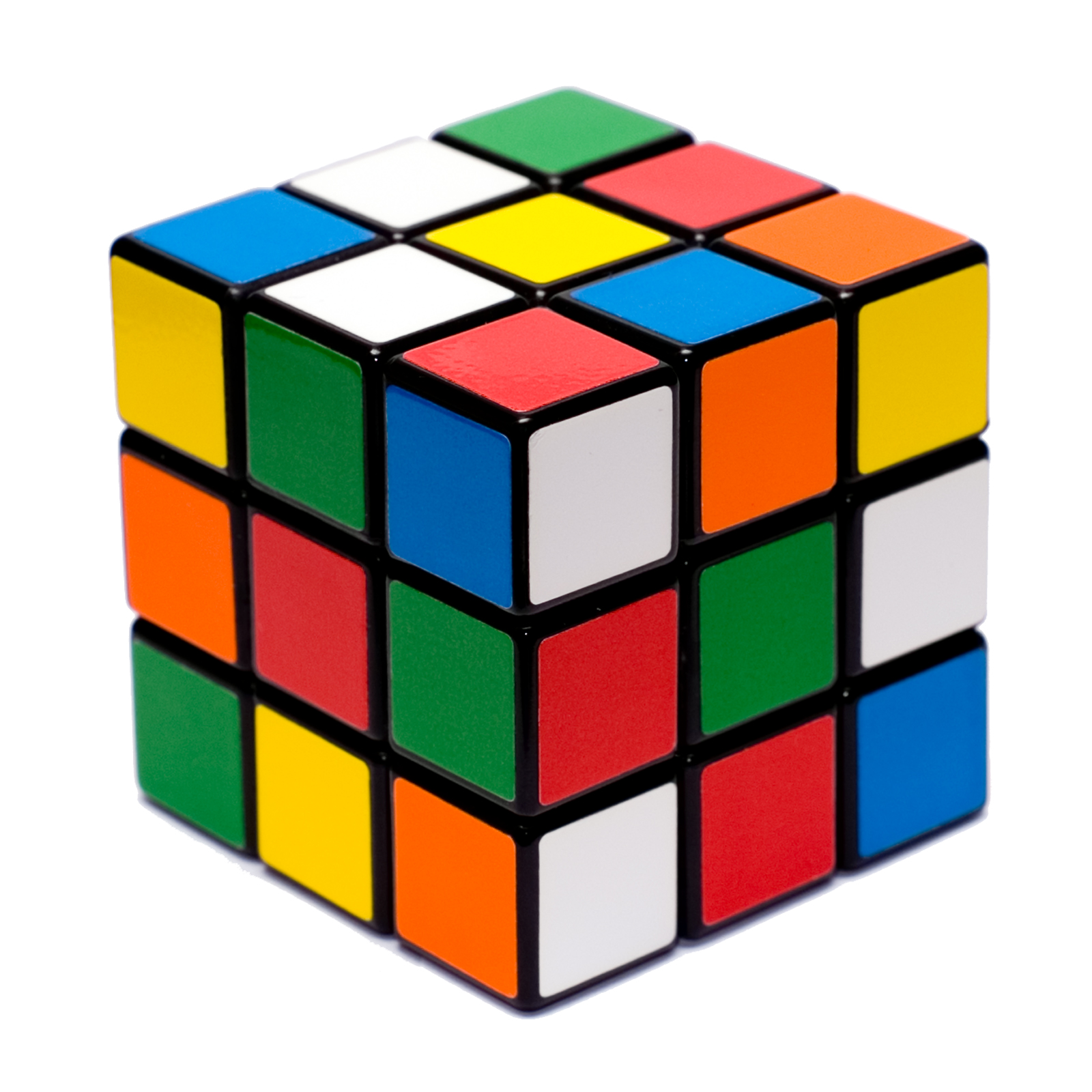
One interesting challenge I solved these days was the “Rubik Cycle”. As explained in the question’s wording, “an interesting property of the Rubik’s Cube is that any sequence of movements, if applied repeatedly, causes the cube to return to its original state (the state it had before the first application of the sequence). For example, after four applications of the sequence B the cube returns to its original state.” The challenge is, given a sequence of movements, to determine the minimum number of complete applications of that sequence to make the cube return to its original state. The input may contain several test cases, each with up to 80 movements.

For you Mathematicians out there, this problem has a direct link with Group Theory. If things like Cyclic Groups, Generators and Rotational Symmetries are your thing, you can probably skip the rest of this post. :) Read this instead:

• The Mathematics of the Rubik’s Cube
• Rubik’s Cube group
• Cyclic group
• How to find the order of a Rubik’s cube algorithm?

Since I’m not acquainted with Group Theory, I decided to code the rotations themselves. I implemented solutions in Python, with and without NumPy, and in C. And found some huge differences in the execution time, which I explore a little bit in the end.

The full source codes are available at my GitHub repository.

Visualizing Rubik’s Cube rotations

My implementation considered each face of the cube as a matrix – specifically, a 3x3 matrix, as we are dealing with the “traditional” Rubik’s Cube here. So, in essence, we are just doing matrix rotations (90º and -90º), but with some important catches, as we are in a 3D space:

1. Each face rotation affects lines and/or columns of adjacent faces.
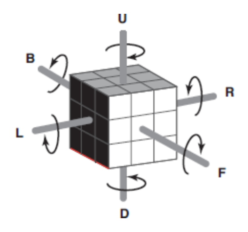
2. We need to pay close attention to how the adjacent faces are affected. For instance, if we rotate a face which has the back (B) face adjacent, we need to remember that this back face is represented with their lines flipped, compared to the other matrices.

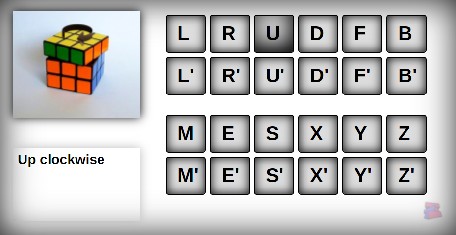
I found it an excellent exercise of 3D space visualization! This website also helped a lot: Ruwix - Rubik’s Cube Notation.

Play with the cube there, and try to imagine each face as a 3x3 matrix. Now visualize where a position [i,j] in a certain face would end up if you rotate a face (the same, or another one) clockwise or counterclockwise. Remeber the catches above!

If you had fun with that, read on! :)

Overview of my algorithms

My solution, in all implementations, follows this general algorithm:

1. Read a line with movements. If there is none, exit.
2. Initialize the cycle counter as 1.
3. For each movement in the line, perform the corresponding matrix rotation.
4. After all the movements are performed, check if the cube is in the initial state.
5. If the cube is not in the initial state, increment the counter and go to line 3.
6. Print the counter’s value.
7. Go to line 1.

The rotation algorithm is as follows:

1. Copy the initial cube state. Not strictly necessary, but it makes the rotations easier, and the time complexity impact is negligible (at least in C, as we’ll see later).
2. Parse the move, and rotate the face and adjacent lines and/or columns accordingly. Use the face copies as sources.

I have also developed and alternative rotation algorithm, which considers the face we are rotating as if it were the front one (i.e. as if we were looking it directly in front of us), with a clever use of face references in the function arguments. That allowed a “generic” rotation algorithm to be used, but some special cases still needed to be taken into consideration, like when the back (B) face was involved. Since it didn’t bring any performance gains, and made the visualization more complicated, I discarded it.

Finally, the validation algorithm does this:

1. The “correct” color of each face (as in the initial cube state) is the value in the middle of each matrix, i.e. position [1,1], as this position doesn’t change during the rotations.
2. Thus, just check if the values of the other positions, in each matrix, matches the center one; if they do, for all the matrices, the cube has returned to the initial state.

I’m sure there are more clever algorithms than these ones I developed, and the purely mathematical solution (applying Group Theory) would be even more efficient. But they got the job done, they were quick to implement and passed the time limit of the challenge (these last two aspects are crucial in a programming challenge). Anyway, I’d love to know your solutions for this challenge: feel free to leave a comment!

Oh and if you are interested in the mathematical solution, take a look here:

MZRG - Order Calculator

Open the page source to view the JavaScript implementation.

Implementation in C

Each face is represented as a 3x3 matrix (I defined a CUBE_SZ constant for that), and each color is a number:

1
2
3
4
5
6

short F[CUBE_SZ][CUBE_SZ] = { { 0, 0, 0 }, { 0, 0, 0 }, { 0, 0, 0 } };  
short U[CUBE_SZ][CUBE_SZ] = { { 1, 1, 1 }, { 1, 1, 1 }, { 1, 1, 1 } };  
short D[CUBE_SZ][CUBE_SZ] = { { 2, 2, 2 }, { 2, 2, 2 }, { 2, 2, 2 } };  
short L[CUBE_SZ][CUBE_SZ] = { { 3, 3, 3 }, { 3, 3, 3 }, { 3, 3, 3 } };  
short R[CUBE_SZ][CUBE_SZ] = { { 4, 4, 4 }, { 4, 4, 4 }, { 4, 4, 4 } };  
short B[CUBE_SZ][CUBE_SZ] = { { 5, 5, 5 }, { 5, 5, 5 }, { 5, 5, 5 } };

The rotations are done through loops which transpose the lines and columns accordingly. For instance, a face rotate in the clockwise direction is like this:

1
2
3
4
5
6

for (j = 0; j <= 2; j += 2) {
  for (i = 0; i < CUBE_SZ; i++) {
    face[i][CUBE_SZ - 1 - j] = face_t[j][i];
    face[j][i] = face_t[CUBE_SZ - 1 - i][j];
  }
}

And the edges of, say, the upper (U) face rotated clockwise would change like this:

1
2
3
4
5
6

for (i = 0; i < CUBE_SZ; i++) {
  B[2][i] = Lt[0][CUBE_SZ - 1 - i];
  L[0][i] = Ft[0][i];
  F[0][i] = Rt[0][i];
  R[0][i] = Bt[2][CUBE_SZ - 1 - i];
}

Notice how I’m using the face copies as sources for the transpositions. In C, these copies can be made efficiently by using memcpy():

1
2

short Ft[CUBE_SZ][CUBE_SZ];
memcpy(Ft, F, sizeof(F));

Finally, the validation is implemented as follows:

1
2
3
4
5
6
7
8

for (short i = 0; i < CUBE_SZ; i++) {
  for (short j = 0; j < CUBE_SZ; j++) {
    if (F[i][j] != F[1][1] || U[i][j] != U[1][1] || D[i][j] != D[1][1] || L[i][j] != L[1][1] || R[i][j] != R[1][1] || B[i][j] != B[1][1])
      return FALSE;
  }
}

return TRUE;

Implementation in Python (without NumPy)

The implementation in Python is very similar to the one in C, so I’ll skip most of the details. One thing worth mentioning, though, is the fact that we don’t have (AFAIK) something similar to memcpy() in C. Therefore, and given the fact that Python works with references internally, to correctly copy the faces to new matrices (avoiding any references to the original ones) I had to do this:

1
2
3
4
5
6

Ft = [[F[x][y] for y in range(len(F[0]))] for x in range(len(F))]
Ut = [[U[x][y] for y in range(len(U[0]))] for x in range(len(U))]
Dt = [[D[x][y] for y in range(len(D[0]))] for x in range(len(D))]
Lt = [[L[x][y] for y in range(len(L[0]))] for x in range(len(L))]
Rt = [[R[x][y] for y in range(len(R[0]))] for x in range(len(R))]
Bt = [[B[x][y] for y in range(len(B[0]))] for x in range(len(B))]

I also discovered deepcopy(), which allowed me to do this instead:

1
2
3
4
5
6

Ft = deepcopy(F)
Ut = deepcopy(U)
Dt = deepcopy(D)
Lt = deepcopy(L)
Rt = deepcopy(R)
Bt = deepcopy(B)

However, deepcopy() was much slower, so I used the former approach.

Implementation in Python (with NumPy)

Using NumPy made the implementation much more elegant and straightforward. And it was a bit faster than my original Python code (except when using PyPy, but we’ll get there).

The matrices were created like this:

1
2
3
4
5
6

f = np.full((3, 3), 0, dtype=int)
u = np.full((3, 3), 1, dtype=int)
d = np.full((3, 3), 2, dtype=int)
l = np.full((3, 3), 3, dtype=int)
r = np.full((3, 3), 4, dtype=int)
b = np.full((3, 3), 5, dtype=int)

The rotations were much simpler, since NumPy offers a rot90() method for this, and we can reference entire lines or columns without an explicit loop. A face rotation can be performed in one line:

1

f = np.rot90(f, -1 if move.isupper() else 1)

And the edges rotation can also be done in one line. For instance, the upper (U) face rotated clockwise is simply:

1

b[2, :], l[0, :], f[0, :], r[0, :] = np.flip(l[0, :]).copy(), f[0, :].copy(), r[0, :].copy(), np.flip(b[2, :]).copy()

How cool is that? :) Oh and notice how I’m using the copy() method: it means I didn’t need to make explicit face copies anymore.

Speed comparison

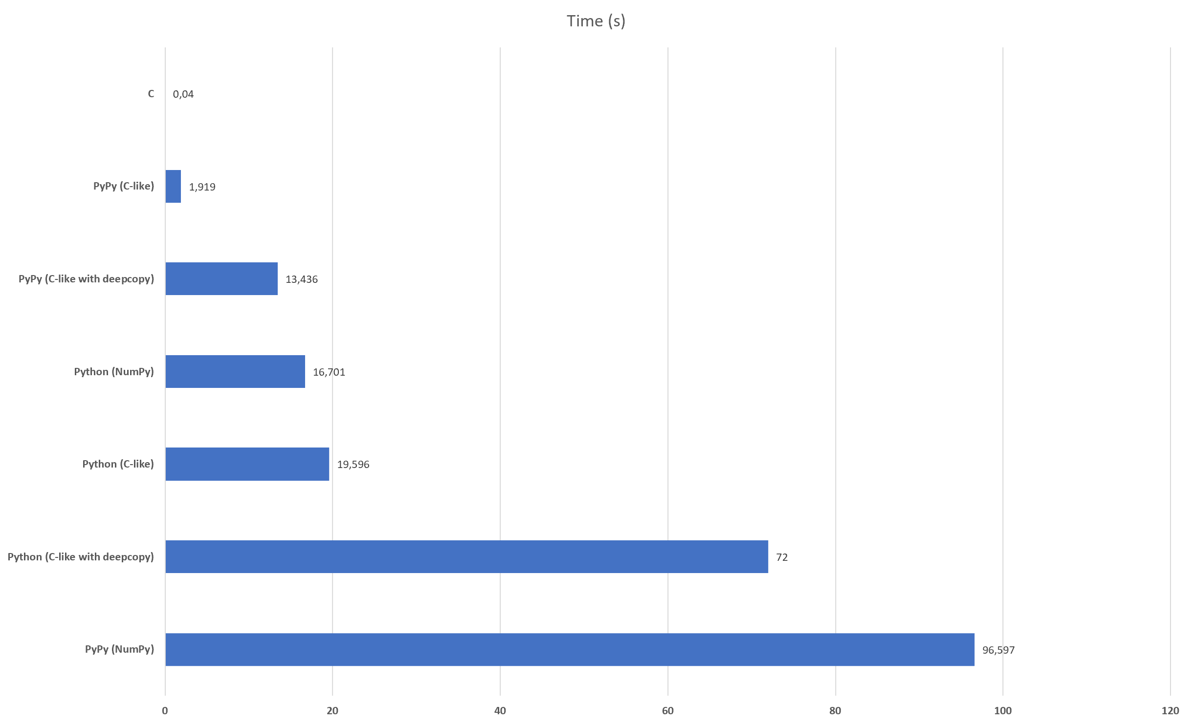
Of course I expected the C implementation to be faster than the Python ones, but not by the amount I found. Remember that the Python implementation (without NumPy) is basically the same as the one in C? So how come it took 19 seconds for an input of 751 test cases (each with up to 80 moves), while the C implementation took less than 1 second for the same input? That’s a difference of almost 20 times!

Other interesting findings: using PyPy, the baseline Python implementation took less than 2 seconds: a 10x speed increase! However, that same PyPy, when running the Python implementation with NumPy, took 1m36s, almost 5.8x slower than the default Python interpreter! Perhaps NumPy doesn’t work well with PyPy for some reason. I also compared how the Python code performs with and without deepcopy().

The chart below summarize all these findings. If you have any insights about why such huge differences are happening, on a lower level, leave a comment!